Fall Detection App: Training Models
Training, optimisation and evaluation of machine learning models with engineered features
In the previous post, we analysed all 3129 activities with 19 features. However, we do not need all of the features. They can be correlated or fully redundant for the prediction.
The dataset 3129 x 19 is not so big that we would not be able to use a more computationally intensive method. In this case, the LOFO library was used.
The LOFO library tests the importance of all features by iteratively removing each feature and checking how the model accuracy changes. If the accuracy drops significantly, that means the feature was important.
Here is the link for the library: LOFO
The LOFO importance and correlation matrix were calculated from the dataset, from which the most important features will be picked.
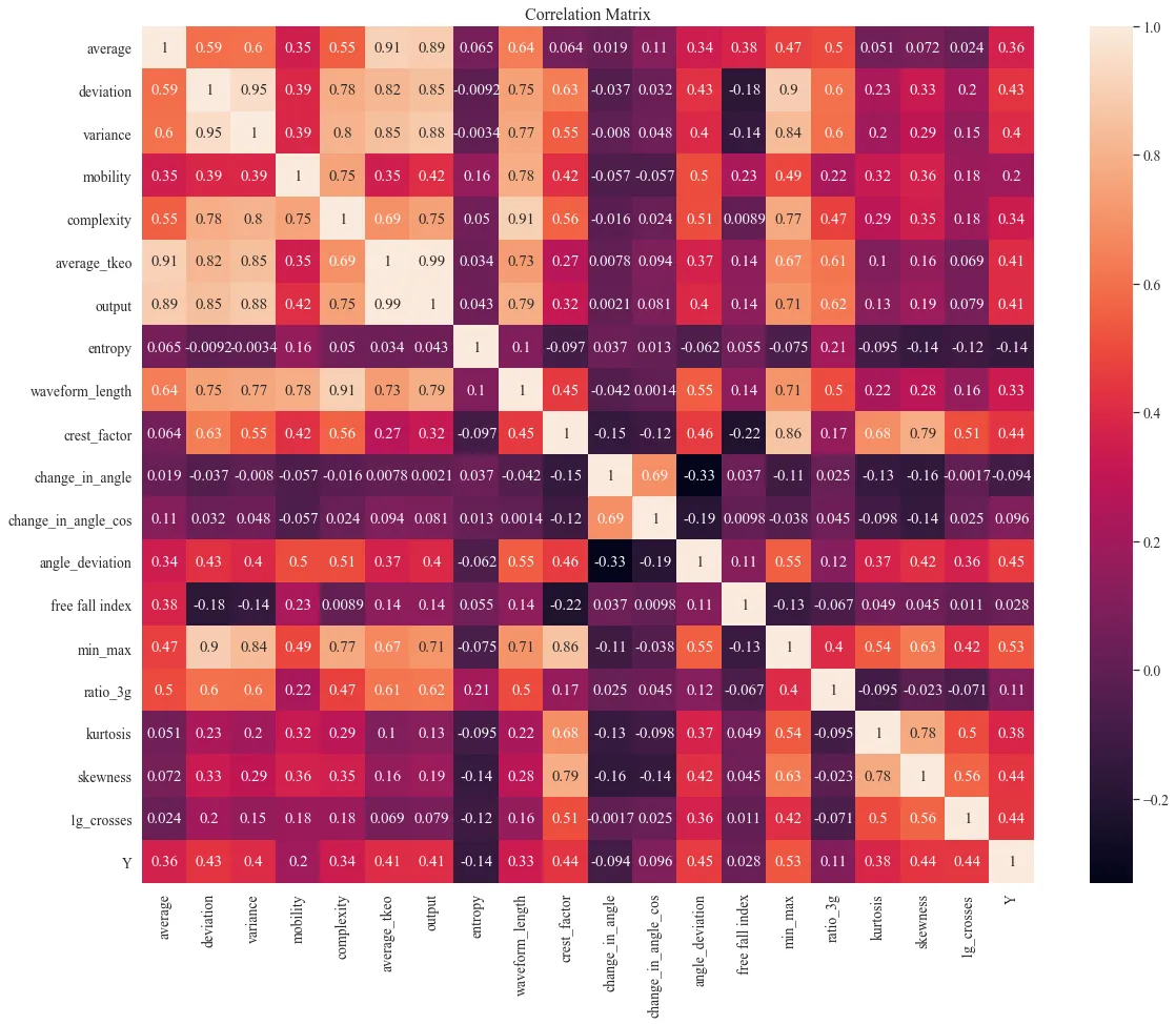
LOFO and correlation matrix
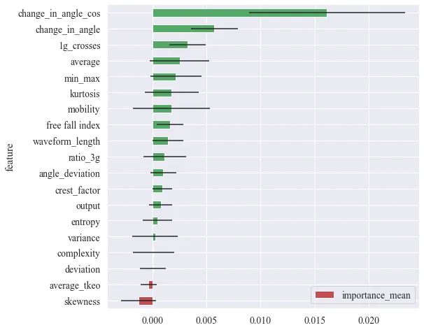
Feature importance results
The change in the angle with cosine is the most important feature. Change in angle is similar but is calculated only from the main event. These features are correlated. However, LOFO does not know to distinguish that, so it will be omitted. Other significant features are 1g crossings, free fall index, kurtosis, and average. There are min-max, mobility and other features, but they are highly correlated with already included features. Moreover, they have a wide range of importance.
Picked features:
- change in angle with cosine
- 1g crossings
- average
- kurtosis
- free fall index
Machine learning —methods
Optimization of the models
Bayesian optimisation is picked as a method of searching for hyperparameters. The bayesian optimisation method uses previous points to narrow down the regions with a high probability of valid parameters within the boundaries, so it avoids blind or grid search of the parameters. From a mathematical perspective, it uses the posterior probability distributions of parameters we want to optimise.
Here is the link for the library: BayesianOptimization
The issue with the library is the lack of support for integers, so in every step, you need to compensate by rounding the number to an integer. The same goes for None, if you want to ignore something, you need to do it on your own in the function.
Random Forest
Random forest generates multiple simpler classification trees to reduce the variance of the final model. Unfortunately, a lot of trees can result in over-fitting. Good performance is easily achievable, because of the nature of the model. The main disadvantage is the high memory requirement, which is essential to avoid for the phone app.
Number of trees, max depth, number of samples for split and minimal samples leaf as parameters were picked to be optimised.
SVM
We also tried the SVM model, which is much more lightweight than RandomForest. However, the SVM can under-perform in our situation, because of a high number of noisy data with a lot of data points. We will use the RBF kernel to minimize the impact of atypical distribution. Parameter C (trade-off to allow some wrong classifications) and Gamma ( how many neighbours will be taken into account) will be optimized.
Machine learning — optimisation function
The optimisation problem is defined as a standalone function, which can use **kwargs (dictionary values). The model type is defined statically before the optimisation. Afterwards, the function is passed into the Bayesian optimizer.
from bayes_opt import BayesianOptimization

"""
  Full code can be found here:
  https://github.com/Foxpace/BeSafeBox_research/blob/master/Research.ipynb
"""

# function for optimisation
def train_model(**kwargs):
    fold_object = StratifiedKFold(n_splits=5, random_state=123, shuffle=True)
    kwargs["random_state"] = 123

    validation_results = []
    validation_f1_results = []
    validation_recall_results = []
    kwargs["class_weight"] = "balanced"

    # to improve range capabilities of the BayesianOptimization
    if "gamma" in kwargs:
        kwargs["gamma"] = 10 ** -kwargs["gamma"]

    # BayesianOptimization does not know to work with discreet values
    if "n_estimators" in kwargs:
        kwargs["n_estimators"] = int(kwargs["n_estimators"] )

    if 'min_samples_leaf' in kwargs:
        kwargs['min_samples_leaf'] = int(kwargs['min_samples_leaf'] )

    if 'min_samples_split' in kwargs:
        kwargs['min_samples_split'] = int(kwargs['min_samples_split'] )

    # to secure pick for no depth limitation - making None available as option
    if "max_depth" in kwargs:
        if kwargs["max_depth"] < 1:
            kwargs["max_depth"] = None
        else:
            kwargs["max_depth"] = int(kwargs["max_depth"])

    clf = clf_object(**kwargs) # creation of the model with hyperparameters

    # k-fold over the data
    for fold, (train, test) in enumerate(fold_object.split(train_X, train_y)):
        clf.fit(train_X[train, :], train_y[train])  # train and performance evaluation of the model
        result_train = clf.score(train_X[train], train_y[train])
        result_test =  clf.score(train_X[test], train_y[test])
        result_val =   clf.score(val_X, val_y)

        predictions_val = clf.predict(val_X)
        f1_val = f1_score(val_y, predictions_val)
        recall_val = recall_score(val_y, predictions_val)

        validation_results.append(result_val)
        validation_f1_results.append(f1_val)
        validation_recall_results.append(recall_val)

        if verbose:
            print("Fold {}.: Train result: {:.2f} %, test result: {:.2f} %, validation result {:.2f} %".format(fold+1, result_train*100, result_test*100, result_val*100))
    if verbose:
        print("")
        print("Average validation accuracy {:.2f} %".format(np.average(validation_results)*100))
        print("Average validation f1 {:.2f} %".format(np.average(validation_f1_results)*100))
        print("Average validation recall {:.2f} %".format(np.average(validation_recall_results)*100))

    return np.average(validation_f1_results) * 100


# RandomForest

# bounds for optimization
pbounds = {'n_estimators': (1, 20),
           'max_depth': (-100, 100),
           'min_samples_leaf': (1, 4.5),
           'min_samples_split': (2, 10.5)
           }
# pick model
verbose = False
clf_object = RandomForestClassifier

# optimization process
optimizer = BayesianOptimization(
    f=train_model,
    pbounds=pbounds,
)
optimizer.maximize(init_points=10, n_iter=100)

# SVM

# bounds for optimization
pbounds = {'C': (0.1, 100), 'gamma': (0, 4)}

clf_object = svm.SVC
optimizer = BayesianOptimization(
    f=train_model,
    pbounds=pbounds,
)
optimizer.maximize(init_points=10, n_iter=40)
Machine learning — results
For RandomForest we obtained:
- trees: 17
- max depth: 90
- minimum sample leaf: 2
- minimum samples for the split: 10
With this, we can obtain overall accuracy of 90.58%, with the precision for the falls 79% and the sensitivity of 89% on the validation data.
For SVM we obtained:
- C: 20.64
- Gamma: 1
With this, we can obtain overall accuracy of 90.42%, with the precision for the falls 77% and the sensitivity of 92% on the validation data.
Both of the results seem promising. However, the data do not represent the real world perfectly. I prepared the dataset of almost 300h real-world accelerometer readings from different environments like taking a bus, exercising in the gym, hiking and others.


